ggplot Linie und Segment

Question

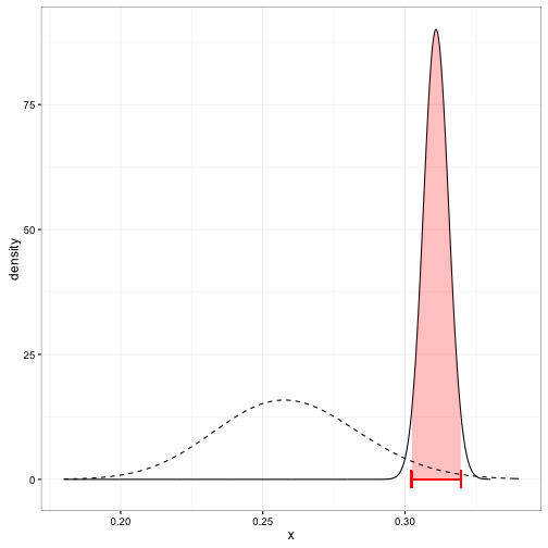
Ich suche ein Grundstück zu erstellen, die auf this one on David Robinson's variance explained blog ähnlich aussieht:

Ich glaube, ich habe es nach unten bis auf die Füllung, die zwischen den glaubhaften Abständen geht und unter der hintere Kurve. Wenn jemand weiß, wie das geht, wäre es schön, einen Rat zu bekommen.

Hier ist ein Beispielcode:

library(ebbr) 
library(ggplot2) 
library(dplyr) 

sample<- data.frame(id=factor(1:10), yes=c(20, 33, 44, 51, 50, 50, 66, 41, 91, 59), 
       total=rep(100, 10)) 

sample<- 
    sample %>% 
    mutate(rate=yes/total) 

pri<- 
    sample %>% 
    ebb_fit_prior(yes, total) 

sam.pri<- augment(pri, data=sample) 

post<- function(ID){ 
    a<- 
    sam.pri %>% 
    filter(id==ID) 

    ggplot(data=a, aes(x=rate))+ 
    stat_function(geom="line", col="black", size=1.1, fun=function(x) 
     dbeta(x, a$.alpha1, a$.beta1))+ 
    stat_function(geom="line", lty=2, size=1.1, 
        fun=function(x) dbeta(x, pri$parameters$alpha,  pri$parameters$beta))+ 
    geom_segment(aes(x=a$.low, y=0, xend=a$.low, yend=.5), col="red", size=1.05)+ 
    geom_segment(aes(x = a$.high, y=0, xend=a$.high, yend=.5), col="red", size=1.05)+ 
    geom_segment(aes(x=a$.low, y=.25, xend=a$.high, yend=.25), col="red", size=1.05)+ 
xlim(0,1) 
} 

post("10") 

Answer 1

Ich mache es in der Regel, indem die Daten erzeugen, die Kurve manuell zu beschreiben, das Hinzufügen Null y-Werte für die min und max des schraffierten Bereich und mit geom_polygon().

library(ebbr) 
library(ggplot2) 
library(dplyr) 

sample <- data.frame(id = factor(1:10), yes = c(20, 33, 44, 51, 50, 50, 66, 41, 91, 59), 
        total = rep(100, 10)) %>% 
    mutate(rate=yes/total) 

pri <- sample %>% 
    ebb_fit_prior(yes, total) 

sam.pri <- augment(pri, data = sample) 

a <- sam.pri %>% 
    filter(id == 10) 

# Make the x values for the shaded region 
x <- seq(from = a$.low, to = a$.high, length.out = 100) 

# Make the y values for the shaded region 
y <- dbeta(x, a$.alpha1, a$.beta1) 

# Make a data.frame for the shaded region, including zeroes 
shaded <- data.frame(x = c(x, a$.high, a$.low), y = c(y, 0, 0)) 

ggplot(data = a, aes(x = rate)) + 
    stat_function(geom = "line", col = "black", size = 1.1, 
       fun = function(x) dbeta(x, a$.alpha1, a$.beta1)) + 
    geom_polygon(data = shaded, aes(x, y), 
       fill = "red", alpha = 0.1) + 
    stat_function(geom = "line", lty = 2, size = 1.1, 
       fun = function(x) dbeta(x, pri$parameters$alpha,  pri$parameters$beta)) + 
    geom_segment(aes(x = a$.low, y = 0, xend = a$.low, yend = 0.5), col = "red", size = 1.05) + 
    geom_segment(aes(x = a$.high, y = 0, xend = a$.high, yend = .5), col = "red", size = 1.05) + 
    geom_segment(aes(x = a$.low, y = .25, xend = a$.high, yend = .25), col = "red", size = 1.05) + 
    xlim(0,1)